class: center middle main-title section-title-4 # Uncertainty .class-info[ **Session 6** .light[PMAP 8921: Data Visualization with R<br> Andrew Young School of Policy Studies<br> Summer 2023] ] --- name: outline class: title title-inv-7 # Plan for today -- .box-2.medium.sp-after-half[Communicating uncertainty] -- .box-4.medium.sp-after-half[Visualizing uncertainty] --- name: communicating class: center middle section-title section-title-2 animated fadeIn # Communicating<br>uncertainty --- layout: true class: title title-2 --- # The Bay of Pigs .pull-left-wide[ <figure> <img src="img/06/bay_of_pigs.jpg" alt="Planning the Bay of Pigs invasion" title="Planning the Bay of Pigs invasion" width="100%"> </figure> ] -- .pull-right-narrow[ .box-inv-2[Joint Chiefs said "fair chance of success"] .box-inv-2[In Pentagon-speak, that meant 3:1 odds of failure] .box-inv-2[25% chance of success!] ] ??? When asked by President John F. Kennedy to assess the CIA invasion plan, the U.S. Joint Chiefs of Staff responded that it had a “fair chance” of success. Kennedy took that as a positive assessment. Instead, the Chiefs meant that they judged the chances of success as “3 to 1 against.” But this was never clarified at the time. Source of story: <https://www.cia.gov/library/center-for-the-study-of-intelligence/csi-publications/books-and-monographs/sherman-kent-and-the-board-of-national-estimates-collected-essays/6words.html> Chart of perceptions and probabilities: <https://www.cia.gov/library/center-for-the-study-of-intelligence/csi-publications/books-and-monographs/psychology-of-intelligence-analysis/fig18.gif/image.gif> --- # Misperceptions of probability .box-inv-2.medium.sp-after[1 in 5 vs. 20%] -- .center[ <img src="06-slides_files/figure-html/unnamed-chunk-1-1.png" width="576" style="display: block; margin: auto;" /> ] --- # Misperceptions of probability .center[ <figure> <img src="img/06/forecast-ut.png" alt="UT Senate 2018 forecast from FiveThirtyEight" title="UT Senate 2018 forecast from FiveThirtyEight" width="90%"> </figure> ] ??? UT Senate 2018 election forecast from FiveThirtyEight --- # Misperceptions of probability .center[ <figure> <img src="img/06/forecast-tx.png" alt="TX Senate 2018 forecast from FiveThirtyEight" title="TX Senate 2018 forecast from FiveThirtyEight" width="90%"> </figure> ] ??? TX Senate 2018 election forecast from FiveThirtyEight --- # Misperceptions of probability .box-inv-2.sp-after[Chance of rain = Probability × Area] -- .pull-left-wide[ <figure> <img src="img/06/rain@4x.png" alt="ZZZ" title="ZZZ" width="100%"> </figure> ] -- .pull-right-narrow[ .box-inv-2[100% chance in<br>1/3 of the city] .box-inv-2[0% chance in<br>2/3 of the city] .box-inv-2[Chance of rain<br>for city = 33%] ] ??? When it doesn't rain, it doesn't mean the forecast was wrong! 30% chance doesn't mean it’ll rain just 30% hard. Average over tons of simulations. Depends on geographic area --- # Misperceptions of probability .center[ <figure> <img src="img/06/coins.jpg" alt="Stack of coins" title="Stack of coins" width="70%"> </figure> ] ??? [Coins](http://www.freestockphotos.biz/stockphoto/8215) --- # Misperceptions of probability .pull-left[ <figure> <img src="img/06/maria2.png" alt="Hurricane Maria NOAA" title="Hurricane Maria NOAA" width="100%"> <figcaption>Hurricane Maria map, NOAA</figcaption> </figure> ] -- .pull-right[ <figure> <img src="img/06/maria1.png" alt="Hurricane Maria NYT" title="Hurricane Maria NYT" width="100%"> <figcaption>Hurricane Maria map, New York Times</figcaption> </figure> ] ??? Or just use a sharpie! --- # The needle .center[ <figure> <img src="img/06/needle.gif" alt="2016 election needle" title="2016 election needle" width="50%"> </figure> ] ??? Extra data is implicitly encoded in aesthetics - temporal sequence of ballot counting – how did Amanda Cox defend this? Via https://www.vis4.net/blog/2016/11/jittery-gauges-election-forecast/ --- # The needle .pull-left[ <figure> <img src="img/06/needle-ga.png" alt="Needle GA-7 2017" title="Needle GA-7 2017" width="100%"> </figure> ] .pull-right[ <figure> <img src="img/06/needle-tweets.png" alt="Twitter reactions to needle" title="Twitter reactions to needle" width="100%"> </figure> ] --- layout: false name: visualizing class: center middle section-title section-title-4 animated fadeIn # Visualizing uncertainty --- layout: true class: title title-4 --- # Problems with single numbers .pull-left[ <img src="06-slides_files/figure-html/animal-weight-bar-1.png" width="100%" style="display: block; margin: auto;" /> ] -- .pull-right[ <img src="06-slides_files/figure-html/animal-weight-points-1.png" width="100%" style="display: block; margin: auto;" /> ] --- # More information is always better .box-inv-4.medium[Avoid visualizing single numbers when you have a whole range or distribution of numbers] -- .box-4[Uncertainty in single variables] -- .box-4[Uncertainty across multiple variables] -- .box-4[Uncertainty in models and simulations] --- # Histograms .box-inv-4[Put data into equally spaced buckets (or bins),<br>plot how many rows are in each bucket] .left-code[ ```r library(gapminder) gapminder_2002 <- gapminder %>% filter(year == 2002) ggplot(gapminder_2002, aes(x = lifeExp)) + geom_histogram() ``` ] .right-plot[ 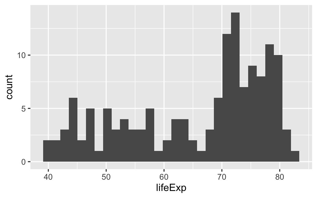 ] --- # Histograms: Bin width .box-inv-4[No official rule for what makes a good bin width] .pull-left-3[ .box-4.small[Too narrow:<br>`binwidth = 0.2`] <img src="06-slides_files/figure-html/hist-too-narrow-1.png" width="100%" style="display: block; margin: auto;" /> ] -- .pull-middle-3[ .box-4.small[Too wide:<br>`binwidth = 50`] <img src="06-slides_files/figure-html/hist-too-wide-1.png" width="100%" style="display: block; margin: auto;" /> ] -- .pull-right-3[ .box-4.small[(One type of) just right:<br>`binwidth = 2`] <img src="06-slides_files/figure-html/hist-just-right-1.png" width="100%" style="display: block; margin: auto;" /> ] --- # Histogram tips .pull-left[ .box-inv-4.small[Add a border to the bars<br>for readability] .box-4.tiny[`geom_histogram(..., color = "white")`] <img src="06-slides_files/figure-html/hist-border-1.png" width="100%" style="display: block; margin: auto;" /> ] -- .pull-right[ .box-inv-4.small[Set the boundary;<br>bucket now 50–55, not 47.5–52.5] .box-4.tiny[`geom_histogram(..., boundary = 50)`] <img src="06-slides_files/figure-html/hist-boundary-1.png" width="100%" style="display: block; margin: auto;" /> ] --- # Density plots .box-inv-4[Use calculus to find the probability of each x value] .left-code[ ```r ggplot(gapminder_2002, aes(x = lifeExp)) + geom_density(fill = "grey60", color = "grey30") ``` ] .right-plot[ 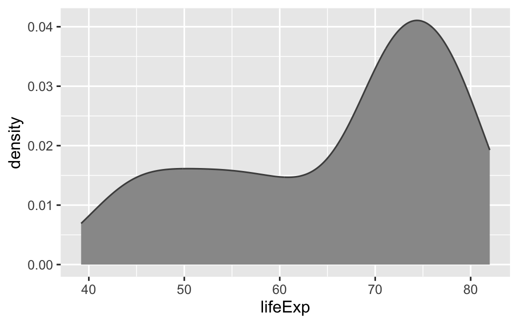 ] --- # Density plots: Kernels and bandwidths .box-inv-4[Different options for calculus change the plot shape] .pull-left-3[ .box-4.small[`bw = 1`] <img src="06-slides_files/figure-html/gaussian-bw-1-1.png" width="100%" style="display: block; margin: auto;" /> ] -- .pull-middle-3[ .box-4.small[`bw = 10`] <img src="06-slides_files/figure-html/gaussian-bw-10-1.png" width="100%" style="display: block; margin: auto;" /> ] -- .pull-right-3[ .box-4.small[`bw = "nrd0"` <small>(default)</small>] <img src="06-slides_files/figure-html/gaussian-bw-auto-1.png" width="100%" style="display: block; margin: auto;" /> ] --- # Density plots: Kernels and bandwidths .box-inv-4[Different options for calculus change the plot shape] .pull-left-3[ .box-4.small[`kernel = "gaussian"`] <img src="06-slides_files/figure-html/gaussian-kernel-gaussian-1.png" width="100%" style="display: block; margin: auto;" /> ] -- .pull-middle-3[ .box-4.small[`"epanechnikov"`] <img src="06-slides_files/figure-html/gaussian-kernel-epanechnikov-1.png" width="100%" style="display: block; margin: auto;" /> ] -- .pull-right-3[ .box-4.small[`"rectangular"`] <img src="06-slides_files/figure-html/gaussian-kernel-rectangular-1.png" width="100%" style="display: block; margin: auto;" /> ] --- # Box plots .box-inv-4[Show specific distributional numbers] .left-code[ ```r ggplot(gapminder_2002, aes(x = lifeExp)) + geom_boxplot() ``` ] .right-plot[ 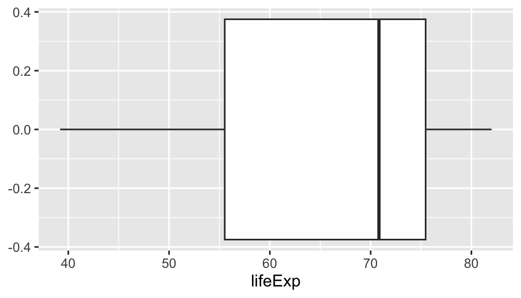 ] --- # Box plots <img src="06-slides_files/figure-html/boxplot-explanation-1.png" width="100%" style="display: block; margin: auto;" /> --- # Violin plots .box-inv-4[Mirror density plot and flip] .box-4.small[Often helpful to overlay other things on it] .left-code[ ```r ggplot(gapminder_2002, aes(x = "", y = lifeExp)) + geom_violin() + geom_boxplot(width = 0.1) ``` ] .right-plot[ 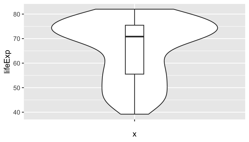 ] ??? <https://xkcd.com/1967/> --- # Uncertainty across multiple variables .box-inv-4.medium.sp-after[Visualize the distribution of a<br>single variable across groups] -- .box-inv-4.medium[Add a `fill` aesthetic or use faceting!] --- # Multiple histograms .box-inv-4[Fill with a different variable] .box-4[This is bad and really hard to read though] .left-code[ ```r ggplot(gapminder_2002, aes(x = lifeExp, fill = continent)) + geom_histogram(binwidth = 5, color = "white", boundary = 50) ``` ] .right-plot[ 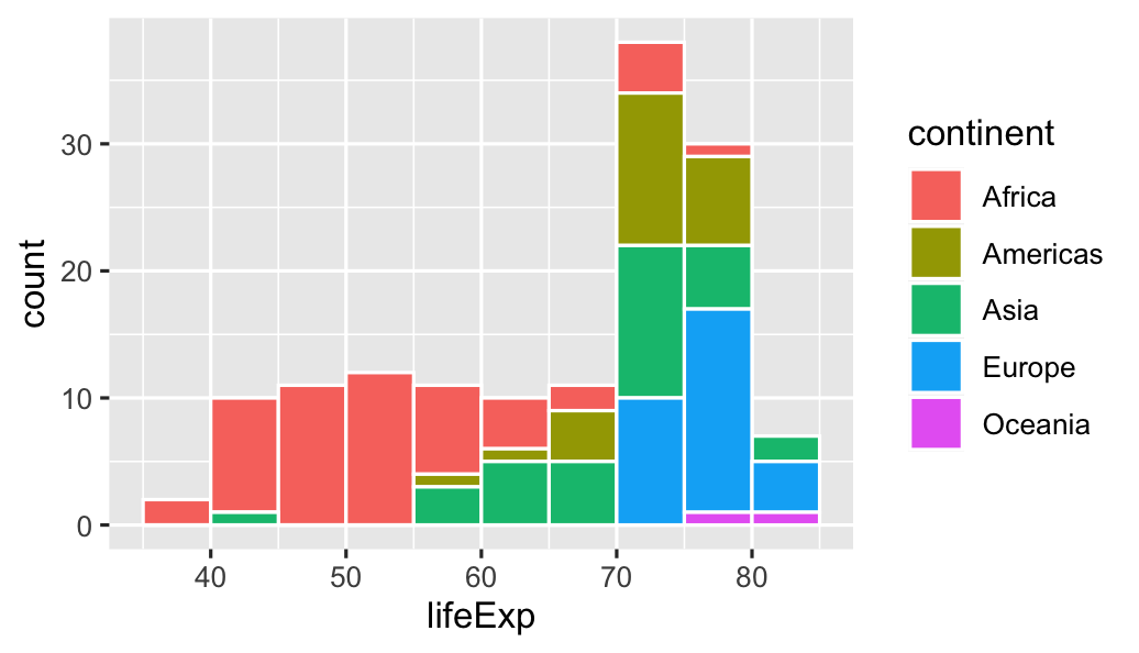 ] --- # Multiple histograms .box-inv-4[Facet with a different variable] .left-code[ ```r ggplot(gapminder_2002, aes(x = lifeExp, fill = continent)) + geom_histogram(binwidth = 5, color = "white", boundary = 50) + guides(fill = "none") + facet_wrap(vars(continent)) ``` ] .right-plot[ 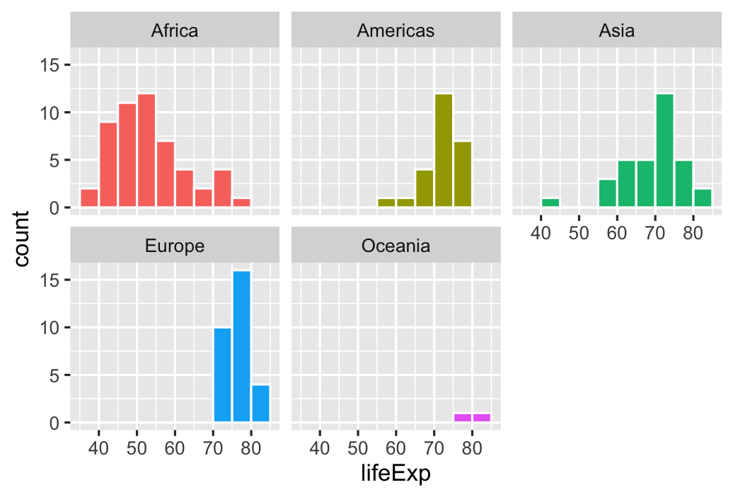 ] --- # Pyramid histograms .left-code.small-code[ ```r gapminder_intervals <- gapminder %>% filter(year == 2002) %>% mutate(africa = ifelse(continent == "Africa", "Africa", "Not Africa")) %>% mutate(age_buckets = cut(lifeExp, breaks = seq(30, 90, by = 5))) %>% group_by(africa, age_buckets) %>% summarize(total = n()) ggplot(gapminder_intervals, aes(y = age_buckets, x = ifelse(africa == "Africa", total, -total), fill = africa)) + geom_col(width = 1, color = "white") ``` ] .right-plot[ 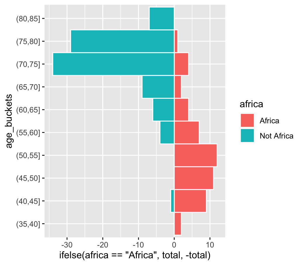 ] ??? There's no way to use `geom_histogram()` to do this, but we can fake it with `geom_col()` --- # Multiple densities: Transparency .left-code[ ```r ggplot(filter(gapminder_2002, continent != "Oceania"), aes(x = lifeExp, fill = continent)) + geom_density(alpha = 0.5) ``` ] .right-plot[ 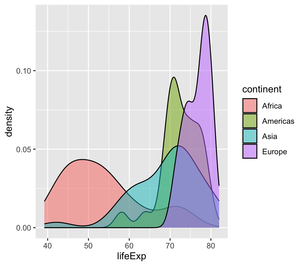 ] --- # Multiple densities: Ridge plots .left-code[ ```r library(ggridges) ggplot(filter(gapminder_2002, continent != "Oceania"), aes(x = lifeExp, fill = continent, y = continent)) + geom_density_ridges() ``` ] .right-plot[ 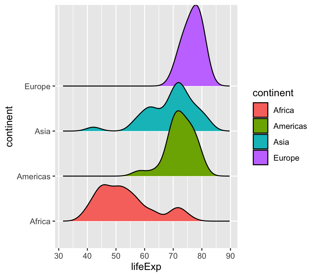 ] --- # Multiple densities: Ridge plots .center[ <figure> <img src="img/06/dwnominate.png" alt="DW-NOMINATE of US House by Party" title="DW-NOMINATE of US House by Party" width="65%"> </figure> ] --- # Multiple geoms: `gghalves` .left-code[ ```r library(gghalves) ggplot(filter(gapminder_2002, continent != "Oceania"), aes(y = lifeExp, x = continent, color = continent)) + geom_half_boxplot(side = "l") + geom_half_point(side = "r") ``` ] .right-plot[ 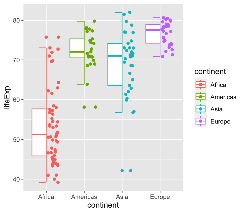 ] --- # Multiple geoms: Raincloud plots .left-code[ ```r library(gghalves) ggplot(filter(gapminder_2002, continent != "Oceania"), aes(y = lifeExp, x = continent, color = continent)) + geom_half_point(side = "l", size = 0.3) + geom_half_boxplot(side = "l", width = 0.5, alpha = 0.3, nudge = 0.1) + geom_half_violin(aes(fill = continent), side = "r") + guides(fill = "none", color = "none") + * coord_flip() ``` ] .right-plot[ 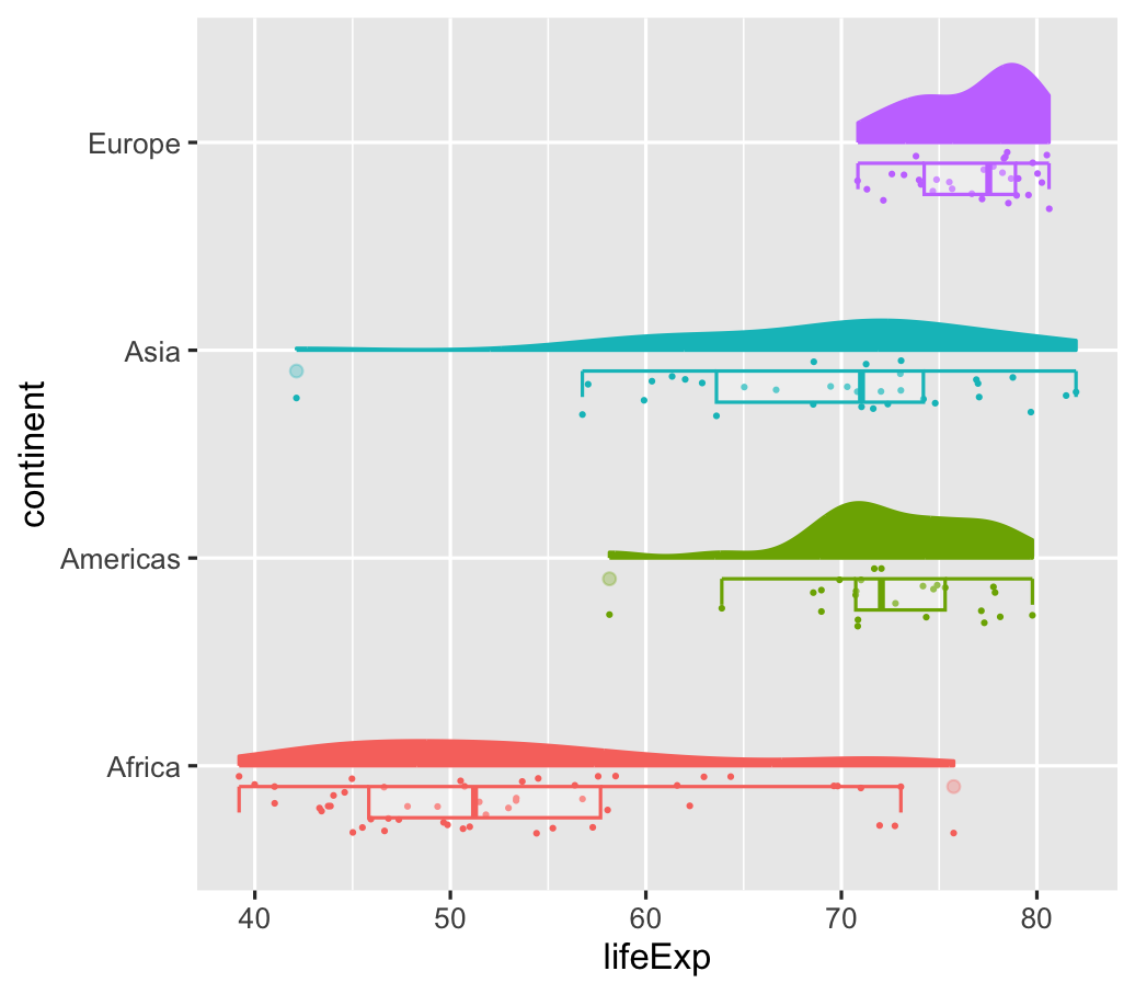 ] --- # Uncertainty in model estimates .box-inv-4[(You'll learn how to make these in the next session)] .center[ <figure> <img src="img/06/1-coefs-bayes.png" alt="Dissertation CSRE coefficient plot" title="Dissertation CSRE coefficient plot" width="60%"> </figure> ] --- # Uncertainty in model estimates .center[ <figure> <img src="img/06/fig-coefs-h3-bayes.png" alt="INGOs and aid coefficient plot" title="INGOs and aid coefficient plot" width="85%"> </figure> ] --- # Uncertainty in model estimates .center[ <figure> <img src="img/06/results-h1-4.png" alt="Why donors donate halfeye plot" title="Why donors donate halfeye plot" width="75%"> </figure> ] --- # Uncertainty in model effects .box-inv-4[(You'll learn how to make these in the next session)] .center[ <figure> <img src="img/06/1-ext-pred.png" alt="Dissertation marginal effects plot" title="Dissertation marginal effects plot" width="75%"> </figure> ] --- # Uncertainty in model outcomes .center[ <figure> <img src="img/06/fivethirtyeight-outcomes.png" alt="FiveThirtyEight model outcomes plot" title="FiveThirtyEight model outcomes plot" width="55%"> <figcaption>FiveThirtyEight's 2018 midterms model outcomes plot</figcaption </figure> ]